-
Global News: Buzz kill? Gen Z less interested in coffee than older Canadians, survey shows
Faculty of Agricultural and Food Sciences, UM Today
-

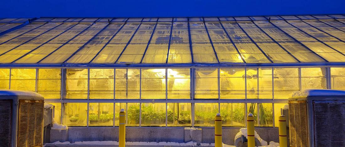
National Post: FuelPositive Announces Strategic Focus on Manitoba, Expanding Network and New Partnerships
Faculty of Agricultural and Food Sciences, UM Today
-
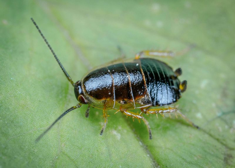
CTV Saskatoon: Saskatoon exterminator says cockroaches live ‘everywhere you go’
Faculty of Agricultural and Food Sciences, UM Today
What we offer
Since our founding in 1906, the Faculty of Agricultural and Food Sciences has continuously evolved to meet the changing needs of our world, embracing new technologies, interdisciplinary collaboration and agile curriculum focused on student success. Our programs of study, unique student experience and researchers are what set us apart. Our partnerships with industry are what help our graduates continue to make change within our community and within the global conversation around food, human health and agriculture.

Departments and School
Centres
Connect with us
Learn more about and contact the people in the Faculty of Agricultural and Food Sciences.
You may also be interested in
Contact us
Dean's Office
Room 256 Agriculture Building
66 Dafoe Road
University of Manitoba (Fort Garry campus)
Winnipeg, MB R3T 2N2 Canada